In this blog, we explore the possibility of using machine learning to reconstruct electroanatomical maps at clinically relevant resolutions using only standard 12-lead electrocardiograms (ECGs) as input. The blog post is also available in Medium.

Heart disease is the leading cause of death in the United States. Every 34 seconds, one person in the US succumbs to cardiovascular disease, and it costs the country approximately $229 billion each year. Most sudden deaths are caused by abnormal electrical rhythms, also known as arrhythmias. In order to diagnose these dangerous conditions, medical professionals turn to the electrocardiogram (ECG). This test is non-invasive, cost-effective, and can distinguish between a wide range of heart conditions.

State-of-the-art methods for non-invasive imaging of cardiac electrical activity often require recordings from multiple locations on the torso and the use of costly medical imaging procedures. In this blog, I explore whether machine learning can be used to reconstruct electroanatomical maps at clinically relevant resolutions using only standard 12-lead electrocardiograms (ECGs) as input.

Basics of electrocardiography

The heart beats thanks to a complex process involving chemistry, electricity, and mechanics. The electrical signal begins at the heart’s natural pacemaker, the SA node, and travels to the AV node, where it is delayed to allow for ventricle filling. From there, it passes through the Purkinje Network, a specialized network for rapid electrical signal conduction, and enters the myocardium via the Purkinje-Muscle Junctions. This triggers the mechanical contraction, which generates an external potential that spreads throughout the body and is measured by the electrocardiogram (ECG).

While there are many ECG recordings available for training machine learning models to classify heart conditions, obtaining full datasets of ECG and spatio-temporal activation maps of the heart is expensive and difficult. To create these maps, a combination of ECG and machine learning is required, using techniques such as data augmentation and synthetic data approaches. By leveraging decades of research on cardiac electrophysiology and training neural networks on detailed simulations, we can gain a better understanding of the heart and its activity.

Data augmentation through detailed cardiac electrophysiology simulations

The goal of this work is to develop a machine learning approach for reconstructing spatio-temporal electroanatomical maps of the myocardium from 12-lead ECGs. To obtain the training data, we follow a synthetic data approach, where we use a detailed cardiac simulation code to generate a large dataset of spatio-temporal activation maps of the heart. At the core of the simulation code is the monodomain model, a system of reaction-diffusion equations that describes the spatiotemporal evolution of the transmembrane voltage $v$ within the myocardium.

where $t$ is time, $C_m$ is the membrane surface capacitance, $\chi$ is the tissue surface area-to-volume ratio, $\boldsymbol{\sigma}$ is the spatially-dependent anisotropic conductivity tensor and $I_{stim}$ is the imposed stimulus. The vector $\boldsymbol{w}$ represents ionic species fluxes through the cell membrane and it is defined by the Ten-Tusscher cell model (Ten-Tusscher 2006), which also defines the non-linear operators $I_{ion}$ and $g$. The dependence of the latter to the $G_{Kr}$ is made explicit for future reference. The Ten-Tusscher model depends on the heart region (endocardial, midmyocardial, and epicardial) as described in . The system above is supplemented with appropriate boundary conditions and initial conditions $v_0$ and $\boldsymbol{w}_0$.

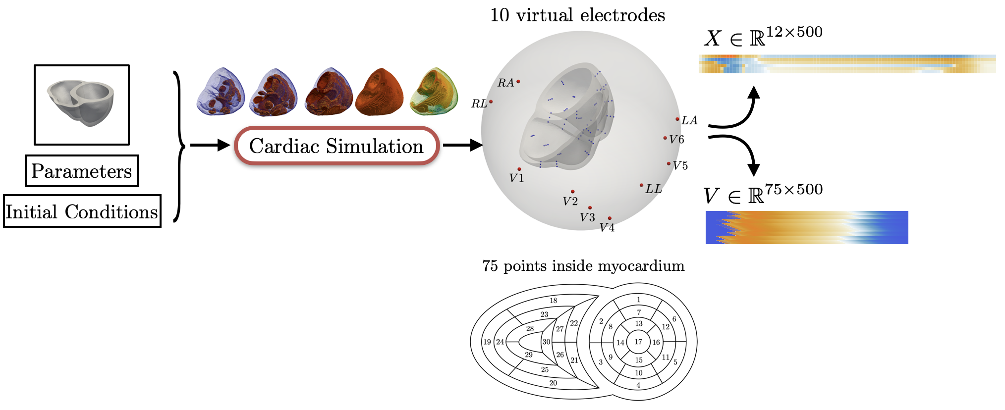
For the recording of the transmembrane voltages within the myocardium, 30 points were selected by hand for each mesh — 17 endocardial points were selected in the left ventricle (LV), corresponding to standard AHA17 segment locations, and 13 points were selected in the right ventricle (RV). From these 30 points, 20 exterior wall points were programmatically identified based on minimum distances from the hand-selected endocardial points, and 25 mid-myocardial points were then found through interpolation. For each simulation performed, simulated transmembrane voltages were recorded for each of the 75 epicardial/midmyocardial/endocardial points. These transmembrane voltages were paired with the ECGs collected above for use in the machine learning classifier.

A wide range of physiological and pathophysiological parameters was considered, including variations in tissue conductivities, maximal conductance $G_{Kr}$ of the rapid delayed rectifier current (0%, or blocked, and 50 % with respect the original value in TenTusscher2006), and basic cycle lengths of (600 ms and 1000 ms). All simulations were performed for 500 ms of simulation time with 200 $\mu$ m resolution meshes and a time-step of 5 $\mu$ s. The ECG and transmembrane voltages were recorded at a resolution of 1 ms. We run each of this parameters combination over a cohort of 15 real patients, and we obtained a total of 16140 simulations. We published this data in the Dataset of Simulated Intracardiac Transmembrane Voltage Recordings and ECG Signals .

Machine learning for Electrocardiography

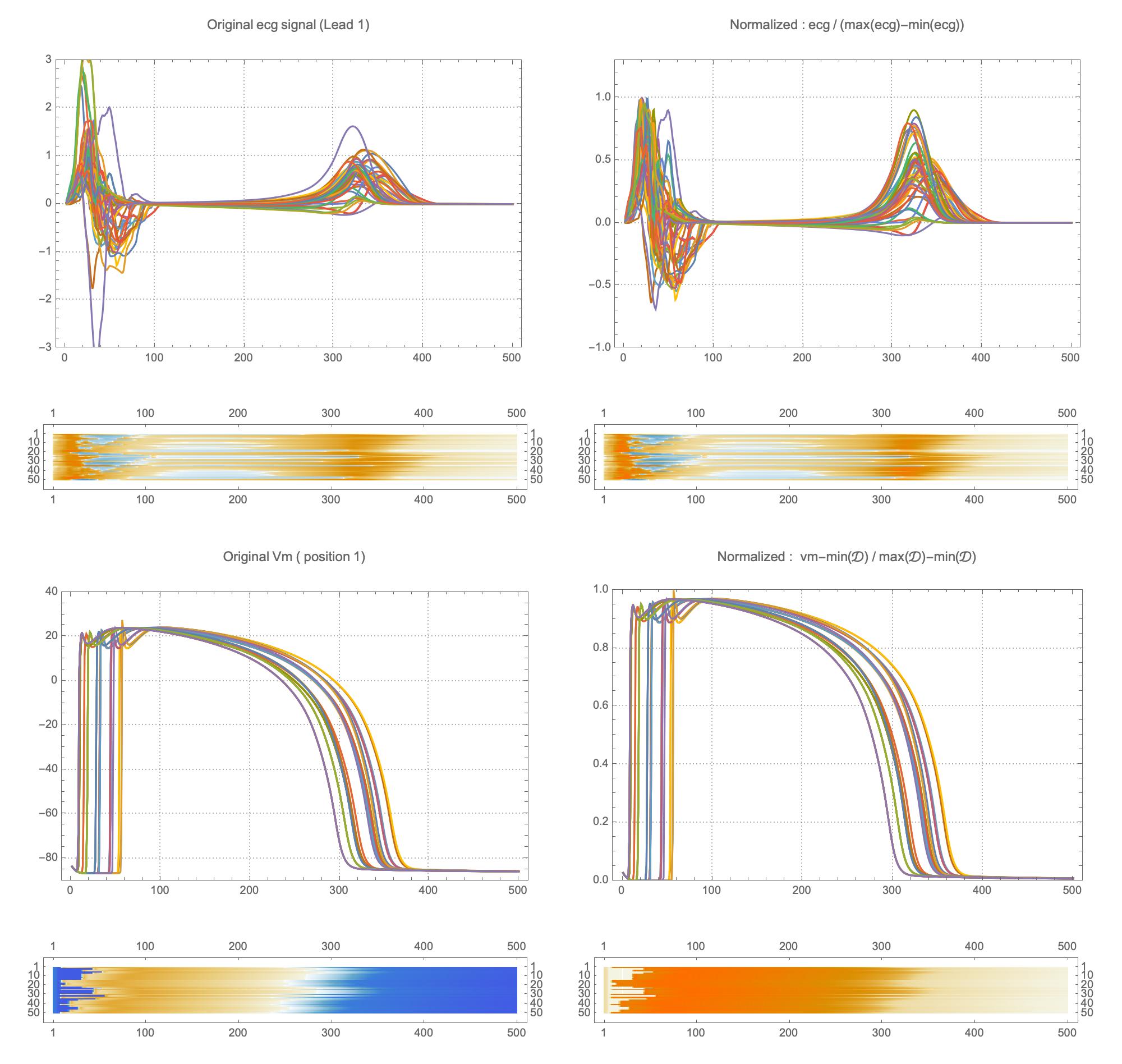
The simulation study described above produced pairs of 12-by-500 $\times$ 1ms ECG signals and 75-by-500 $\times$ 1ms transmembrane voltage signals. For the sake of notation, those signals are represented as matrices $X \in {\mathbb{R}}^{12\times 500}$ and $V \in {\mathbb{R}}^{75 \times 500}$, respectively. The activation time vector $A \in {\mathbb{R}}^{75}$, corresponding to the initial activation time at each myocardial recording location, is defined as $A_i= \min_{j} V_{ij} > 0$. Two machine learning tasks were considered in this work: Task I (activation map reconstruction), which involved reconstructing $A \in {\mathbb{R}}^{75}$ from $X \in {\mathbb{R}}^{12\times 500}$, and Task II (transmembrane potential reconstruction), which involves reconstructing $V \in {\mathbb{R}}^{75\times 500}$ given $X \in {\mathbb{R}}^{12\times 500}$.

These tasks can be regarded as sequence-to-sequence prediction problems, where the goal is to transform a 500-length sequence of 12 dimensional vectors into a sequence of 75 dimensional vectors. In this work, where reconstruction was considered over 75 intracardiac positions, the best results were achieved using 1D CNN architectures inspired by the SqueezeNet model (Iandola 2016). Two different networks were considered:

• Network 1 (for Task 1) : Network I was constructed using SqueezeNet (with 1 dimensional kernels) with a stride of size 2 in the first convolutional layer and max pooling layers to progressively reduce the temporal dimension. Additional convolutional layers were added at the end to reduce the output dimension to ${\mathbb{R}}^{75}$. The total number of parameters in the network is 486,657.
• Network 2 (for Task 2) : Network II was constructed using SqueezeNet (with 1 dimensional kernels). Additional convolutional layers were added at the end to produce outputs of dimension ${\mathbb{R}}^{75\times 500}$. The total number of parameters in the network is 392,907.

The considered network architectures allow for both temporal and spatial information derived from the ECG signal to be combined and reorganized in a nonlinear way. For training the networks, each $X \in {\mathbb{R}}^{12\times 500}$ tensor was normalized so that $\max_{j}(X_{ij})-\min_{j}(X_{ij}) = 1, \forall i \in {1,\dots, 12}$. To train Network II, each $V \in {\mathbb{R}}^{75 \times 500}$ was normalized so that the value range was $[0,1]$. The dataset was randomly split into training and validation subsets containing 95% and 5% of the samples, respectively.

The reconstruction obtained by Network 1 incurs an error of 1.66 msec over all 75 recording points in the validation set with a mean standard deviation of 1.49 msec. These results show that Network I is able to reconstruct the activation map over the validation set of simulated data. In particular, the algorithm is able to capture and reproduce both septal and transmural activation times in cardiac tissue.

The reconstruction results obtained with Network 2 for the validation ECG shows an example of reconstructed transmembrane voltage compared with reference simulated result at myocardial recording point $1$. Similar results were obtained for points $17$ and $67$. The corresponding activation time vector $A \in {\mathbb{R}}^{75}$ is computed from $V \in {\mathbb{R}}^{75\times 500}$.

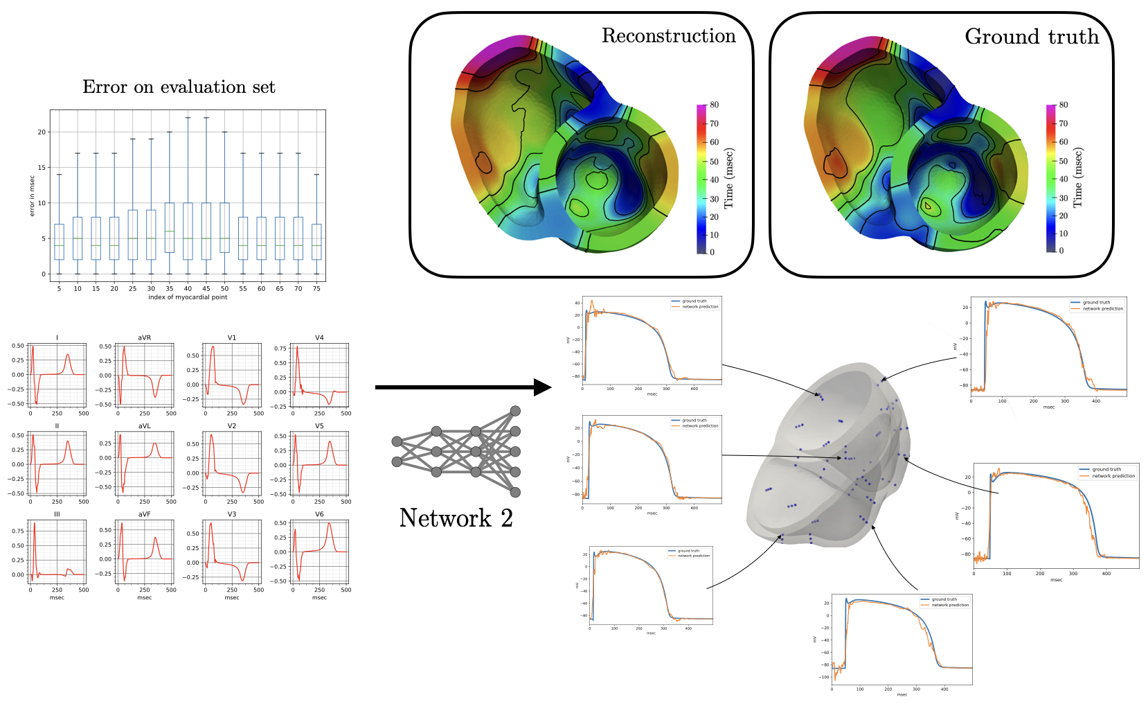
The derived activation times are slightly slower compared to ground truth. Specifically, the mean error in the reconstruction of activation times using Network II for all points in the validation test is 6.5 msec with a mean standard deviation of 6.65 msec. The error is higher than in Network I, and is not surprising since in this case the reconstruction is not targeting the activation map itself but rather the whole temporal evolution of the transmembrane voltage within the myocardium.

Conclusion

The combination of data-augmentation through detailed simulations and machine learning has the potential to significantly improve the accuracy and effectiveness of medical imaging. As researchers continue to explore these techniques, we can expect to see further advancements in the diagnosis and treatment of a wide range of diseases, including heart disease.